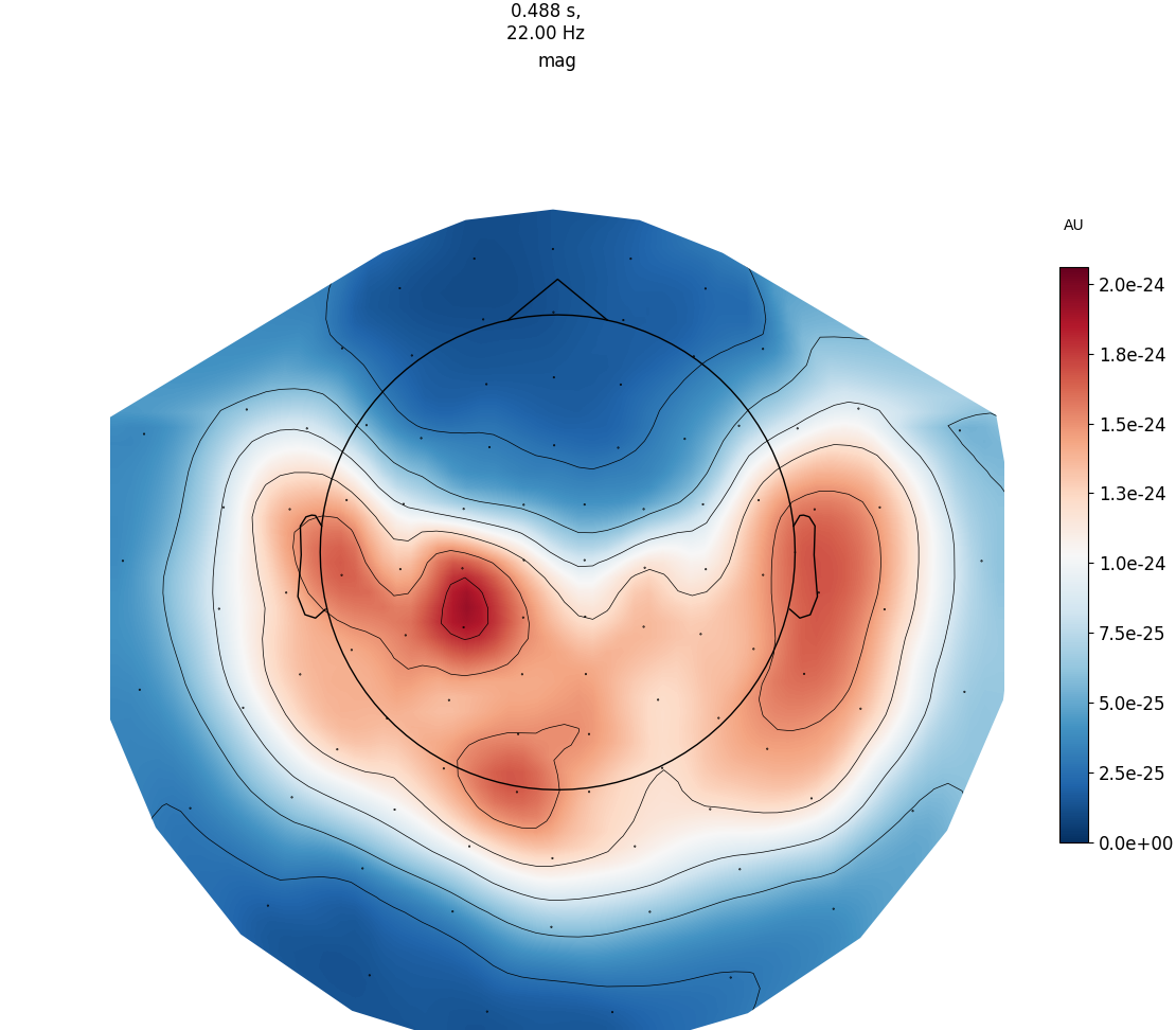
Python-MNE：Python-MNE全套教程（官网翻译）-入门05：关于传感器位置

本教程描述了如何读取和绘制传感器位置，以及MNE-Python如何处理传感器的物理位置。像往常一样，我们将从导入我们需要的模块开始：

from pathlib import Path

import matplotlib.pyplot as plt
import numpy as np

import mne

关于montage和layout（蒙太奇和传感器布局）

montage包含3D传感器位置(x, y, z以米为单位)，可以分配给现有的EEG/MEG数据。通过指定传感器相对于大脑的位置，蒙太奇在计算正向解和逆估计中起着重要作用。

相反，layout是传感器位置的理想化二维表示。它们主要用于在拓扑图中排列单个传感器子图，或用于显示上面观的传感器的近似相对排列。

注意，如果专门处理eeg数据，使用montage更好。理想化的montage，例如由制造商提供的那些，通常被称为template montage（模板）。

使用内置的montage

MEG传感器的三维坐标包含在MEG系统的原始记录中。它们在加载时自动存储在Raw对象的info属性中。而由于头部形状的不同，eeg电极的位置变化很大。许多EEG系统的模板montage都包含在MNE-Python中，可以通过使用mne.channels. get_builtin_montage()来获取：

1
2
3

builtin_montages = mne.channels.get_builtin_montages(descriptions=True)
for montage_name, montage_description in builtin_montages:
    print(f"{montage_name}: {montage_description}")

standard_1005: Electrodes are named and positioned according to the international 10-05 system (343+3 locations)
standard_1020: Electrodes are named and positioned according to the international 10-20 system (94+3 locations)
standard_alphabetic: Electrodes are named with LETTER-NUMBER combinations (A1, B2, F4, …) (65+3 locations)
standard_postfixed: Electrodes are named according to the international 10-20 system using postfixes for intermediate positions (100+3 locations)
standard_prefixed: Electrodes are named according to the international 10-20 system using prefixes for intermediate positions (74+3 locations)
standard_primed: Electrodes are named according to the international 10-20 system using prime marks (‘ and ‘’) for intermediate positions (100+3 locations)
biosemi16: BioSemi cap with 16 electrodes (16+3 locations)
biosemi32: BioSemi cap with 32 electrodes (32+3 locations)
biosemi64: BioSemi cap with 64 electrodes (64+3 locations)
biosemi128: BioSemi cap with 128 electrodes (128+3 locations)
biosemi160: BioSemi cap with 160 electrodes (160+3 locations)
biosemi256: BioSemi cap with 256 electrodes (256+3 locations)
easycap-M1: EasyCap with 10-05 electrode names (74 locations)
easycap-M10: EasyCap with numbered electrodes (61 locations)
easycap-M43: EasyCap with numbered electrodes (64 locations)
EGI_256: Geodesic Sensor Net (256 locations)
GSN-HydroCel-32: HydroCel Geodesic Sensor Net and Cz (33+3 locations)
GSN-HydroCel-64_1.0: HydroCel Geodesic Sensor Net (64+3 locations)
GSN-HydroCel-65_1.0: HydroCel Geodesic Sensor Net and Cz (65+3 locations)
GSN-HydroCel-128: HydroCel Geodesic Sensor Net (128+3 locations)
GSN-HydroCel-129: HydroCel Geodesic Sensor Net and Cz (129+3 locations)
GSN-HydroCel-256: HydroCel Geodesic Sensor Net (256+3 locations)
GSN-HydroCel-257: HydroCel Geodesic Sensor Net and Cz (257+3 locations)
mgh60: The (older) 60-channel cap used at MGH (60+3 locations)
mgh70: The (newer) 70-channel BrainVision cap used at MGH (70+3 locations)
artinis-octamon: Artinis OctaMon fNIRS (8 sources, 2 detectors)
artinis-brite23: Artinis Brite23 fNIRS (11 sources, 7 detectors)
brainproducts-RNP-BA-128: Brain Products with 10-10 electrode names (128 channels)

这些内置的EEG montage可以通过mne.channels. make_standard_montage加载：

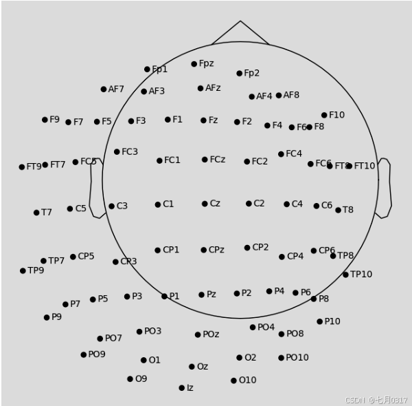
1 2	easycap_montage = mne.channels.make_standard_montage("easycap-M1") print(easycap_montage)

<DigMontage | 0 extras (headshape), 0 HPIs, 3 fiducials, 74 channels>

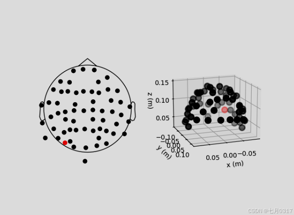
montage对象有一个在2D或3D中可视化传感器位置的绘图方法:

1
2
3

easycap_montage.plot()  # 2D
fig = easycap_montage.plot(kind="3d", show=False)  # 3D
fig = fig.gca().view_init(azim=70, elev=15)  # set view angle for tutorial

加载后，可以使用set_montage方法将蒙太奇应用于数据，例如raw. set_montage()，epochs. set_montage()。这只适用于eeg通道名称对应于montage中的那些数据。
可以通过plot_sensors()方法可视化传感器位置。通过将montage名称直接传递给set_montage()方法，可以跳过手动蒙太奇加载步骤。

这里我们加载了一些非常规的sample数据，以展示手动用已有的文件设置montage，适用于eeg通道名称和内置montage不对应的情况。

ssvep_folder = mne.datasets.ssvep.data_path()
ssvep_data_raw_path = (
    ssvep_folder / "sub-02" / "ses-01" / "eeg" / "sub-02_ses-01_task-ssvep_eeg.vhdr"
)
ssvep_raw = mne.io.read_raw_brainvision(ssvep_data_raw_path, verbose=False)

# Use the preloaded montage
ssvep_raw.set_montage(easycap_montage)
fig = ssvep_raw.plot_sensors(show_names=True)

# Apply a template montage directly, without preloading
ssvep_raw.set_montage("easycap-M1")
fig = ssvep_raw.plot_sensors(show_names=True)

注意，通过plot_sensors()创建的图形可能比easycap_montage.plot()的结果包含更少的传感器。这是因为montage包含了为EEG系统定义的所有通道；但并不是所有的记录都必须使用所有可能的通道。因此，将montage应用于实际的EEG数据集时，有关数据中实际不存在的传感器的信息被删除。

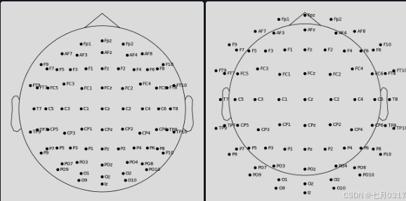
像EEGLAB一样绘制2D传感器位置

如果你喜欢使用10-20个conventions来绘制头部圆圈，可以传递sphere=’ EEGLAB ‘，注意，因为我们在这里使用的数据不包含Fpz频道，所以它的假定位置是自动近似的。：

1	fig = ssvep_raw.plot_sensors(show_names=True, sphere="eeglab")

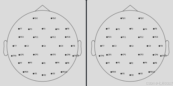
手动控制2D通道投影

通道在2D空间中的位置是通过将其实际的3D位置投影到球体上，然后将球体投影到平面上来获得的。默认情况下，使用原点为(0,0,0)，半径为0.095米(9.5厘米)的球体。你可以通过在任何绘制2D通道的函数中传递单个值作为sphere参数来使用不同的球体半径：

1 2	fig1 = easycap_montage.plot() # default radius of 0.095 fig2 = easycap_montage.plot(sphere=0.07)

为了不仅改变半径，还改变球体原点，传递一个(x, y, z, radius)元组作为球体参数

1	fig = easycap_montage.plot(sphere=(0.03, 0.02, 0.01, 0.075))

读取传感器数字文件

在示例数据中，传感器位置已经在Raw对象的info属性中可用。因此，我们可以使用plot_sensors()直接从Raw对象绘制传感器位置，它提供了与montage.plot()相似的功能。

此外，plot_sensors()支持按类型选择通道，默认情况下，raw.info[‘bads’]中列出的通道将被绘制为红色，并在现有的Matplotlib Axes对象中绘制，因此通道位置可以很容易地作为多面板图中的子图添加：

sample_data_folder = mne.datasets.sample.data_path()
sample_data_raw_path = sample_data_folder / "MEG" / "sample" / "sample_audvis_raw.fif"
sample_raw = mne.io.read_raw_fif(sample_data_raw_path, preload=False, verbose=False)

fig = plt.figure()
ax2d = fig.add_subplot(121)
ax3d = fig.add_subplot(122, projection="3d")
sample_raw.plot_sensors(ch_type="eeg", axes=ax2d)
sample_raw.plot_sensors(ch_type="eeg", axes=ax3d, kind="3d")
ax3d.view_init(azim=70, elev=15)

注意，当使用set_montage()设置montage时，测量信息在两个地方更新（chs和dig条目都被更新）除了电极位置外，dig还可能包含HPI、基准点或头部形状点信息。

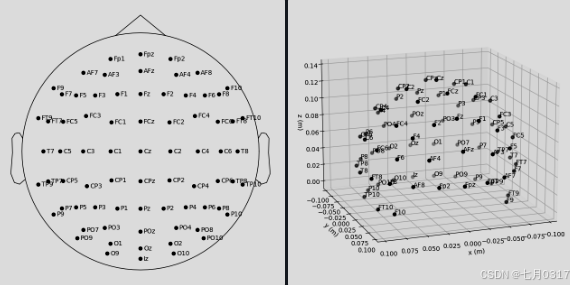
传感器3D表面渲染的可视化

用一个新函数，如下所示：

fig = mne.viz.plot_alignment(
    sample_raw.info,
    dig=False,
    eeg=False,
    surfaces=[],
    meg=["helmet", "sensors"],
    coord_frame="meg",
)
mne.viz.set_3d_view(fig, azimuth=50, elevation=90, distance=0.5)

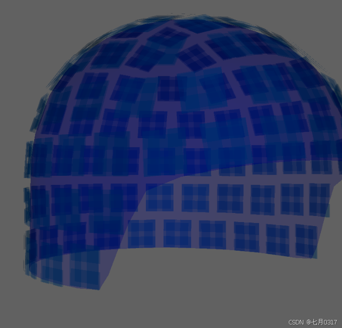
注意，plot_alignment()需要一个Info对象，并且还可以渲染头皮，头骨和大脑的MRI表面（通过将带有’head’， ‘outer_skull’或’brain’键名的字典传递给surfaces参数）。这使得该函数对于评估坐标坐标系转换很有用。

关于layout文件的使用

与montage类似，许多layout文件都包含在MNE-Python中，它们存储在mne/channels/data/layouts文件夹中：

layout_dir = Path(mne.__file__).parent / "channels" / "data" / "layouts"
layouts = sorted(path.name for path in layout_dir.iterdir())
print("\n" "BUILT-IN LAYOUTS\n" "================")
print("\n".join(layouts))

BUILT-IN LAYOUTS
CTF-275.lout
CTF151.lay
CTF275.lay
EEG1005.lay
EGI256.lout
GeodesicHeadWeb-130.lout
GeodesicHeadWeb-280.lout
KIT-125.lout
KIT-157.lout
KIT-160.lay
KIT-AD.lout
KIT-AS-2008.lout
KIT-UMD-3.lout
Neuromag_122.lout
Vectorview-all.lout
Vectorview-grad.lout
Vectorview-grad_norm.lout
Vectorview-mag.lout
biosemi.lay
magnesWH3600.lout

要加载布局文件，可以使用mne.channels.read_layout函数。然后可以使用它的plot方法可视化布局：

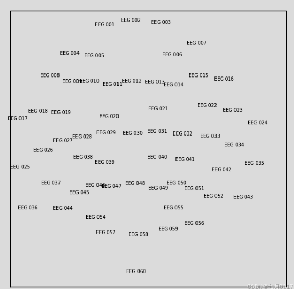
与用于从Raw对象中选择通道的picks参数类似，Layout对象的plot()方法也有一个picks参数。然而，由于布局只包含有关传感器名称和位置信息，没有类型信息，所以只支持按索引选择通道，而不是按名称或类型。在下面的示例中，我们使用numpy.where()找到所需的索引；使用mne.pick_channels()或mne.pick_types()按名称或类型进行选择。

1	biosemi_layout = mne.channels.read_layout("biosemi")

1 2	midline = np.where([name.endswith("z") for name in biosemi_layout.names])[0] biosemi_layout.plot(picks=midline)

如果你有一个包含传感器位置的Raw对象，你可以用mne.channels.make_eeg_layout()或mne.channels.find_layout()创建一个Layout对象。

1
2
3

layout_from_raw = mne.channels.make_eeg_layout(sample_raw.info)
# same result as mne.channels.find_layout(raw.info, ch_type='eeg')
layout_from_raw.plot()

注意，没有相应的make_meg_layout()函数，因为传感器位置在MEG系统中是固定的，不像在EEG中，传感器帽会变形以紧贴特定的头部。因此，对于给定的系统，MEG布局是permanent的，所以可以简单地使用mne.channels.read_layout()加载它们，或者使用带有ch_type参数的mne.channels.find_layout()如前面为EEG演示的那样)。

Python-MNE教程

本文采用署名-非商业性使用-相同方式共享 4.0 国际许可协议，转载请注明出处。